
In 2006, Jeffrey Row and Gabriel Blouin-Demers published a Copeia paper boldly titled “Kernels Are Not Accurate Estimators of Home-range Size for Herpetofauna.” This tutorials based on some code I created to follow their advice in my own studies. In addition, the code below will help you learn to create minimum convex polygons and kernel densitiy estimates in R, even if you don't plan to create a custum smoothing value. MCPs and KDEs can also be used for other anlyses outside of home range analysis, but the methods here work regardless of your intended purpose.
The package adehabitatHR is the go-to package for home range analysis in R. This is a newer and more specialized version of the old adehabitat. Commands are in blue, comments in pink followed by a #, and output in blockquotes or images.
library(adehabitatHR) #load package
Go ahead and load your tracking data. If you use the file choose () command, note that the popup box is often minimized, so you have to look for it. You can call it whatever you want, but I called mine “all.telemetry.” My data is setup so that I have three columns: Snake ID, Easting, and Northing. The Easting and Northing are my GPS coordinates in UTM format. Because my snakes have IDs and not names, I turn their values into categories.
Here’s what my data looks like (with real numbers instead of xxxx):
all.telemetry <- read.csv(file.choose()) #load all telemetry data for H. plat
all.telemetry$SnakeID <- as.factor(all.telemetry$SnakeID) #turn first column into categorical data
head(all.telemetry)
SnakeID Easting Northing
1 605xxxx 478xxxx
2 605xxxx 478xxxx
3 605xxxx 478xxxx
4 605xxxx 478xxxx
5 605xxxx 478xxxx
6 605xxxx 478xxxx
Because I suck at R, let’s look at each snake individually. Maybe as I get better I’ll figure out how to do this for the entire dataset, but for now, we will select a single snake (Snake 1) to analyze. The double = tells R to only include rows with a value of 1 in the first column. (2019 update: I no longer suck at R, but who has time to update old code? This still works, it's just not as efficient or pretty as it could be... so it goes).
s1<- subset(all.telemetry,SnakeID==1) #only look at Snake #1's data
Next, we use the SpatialPoints command from adehabitatHR to turn the easting and northing data into actual GPS coordinates. Remember that functions (commands) in R are case sensitive. The [2:3] tells R to apply the SpatialPoints function only to the second and third columns.
s1xy<- SpatialPoints(s1[2:3]) #turn the xy data into coordinates
Now we will calculate the 100% minimum convex polygon, used to represent the home range of the snake. $area is needed to pull out actual value.
mcp(s1xy, percent = 100) #view all the mcp data
object of class "SpatialPolygonsDataframe" package (sp):
Number of spatial polygons: 1
variables measured:
id area
a a 10.41575
mcp(s1xy, percent = 100)$area #extract just the mcp area
[1] 10.41575
Now we can save this value to use later.
s1_homerange <- mcp(s1xy,percent=100)$area #save the 100% minimum convex polygon value as a variable
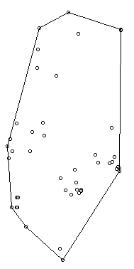
Ok, so now let's view the MCP. We graph the home range of Snake 1, and then add the radio-telemetry locations on top. The pch argument tells R to plot the radio-telemetry locations as circles, and cex controls how big they are. add=TRUE tells R to put the circles on top of the figure that is currently being displayed.
plot(mcp(s1xy,percent=100)) #graph the 100% mcp
plot(s1xy,pch=1,cex=.75,add=TRUE) #add the data points on top
s1_homerange <- mcp(s1xy,percent=100)$area #save the 100% minimum convex polygon value as a variable
Ok, so now let's view the MCP. We graph the home range of Snake 1, and then add the radio-telemetry locations on top. The pch argument tells R to plot the radio-telemetry locations as circles, and cex controls how big they are. add=TRUE tells R to put the circles on top of the figure that is currently being displayed.
plot(mcp(s1xy,percent=100)) #graph the 100% mcp
plot(s1xy,pch=1,cex=.75,add=TRUE) #add the data points on top
So we now have the MCP, and we visualized it to make sure there were no mistakes. Let’s make a utilization distribution (kernel), setting the smoothing factor to “href.” This is actually the default option, so you can leave the h=”href” part out if you want to. Once you create the UD, you can view it in raster form (yuck) with image(ud).
ud <- kernelUD(s1xy,h="href") #calculate and save the utilization distribution
ud <- kernelUD(s1xy,h="href") #calculate and save the utilization distribution

Now we will get something we actually care about, the 95% UD/kernel density. To do that, we can use the getverticeshr command. Why does the most important function have such an unintuitive name? Who knows. The kernel.area command isn’t needed for what we are doing, but it’s nice info to have, so I like to include it.
ud <- kernelUD(s1xy,h="href") #calculate and save the utilization distribution
ver <- getverticeshr(ud,percent=95)$area #find and save the 95% utilization distribution
kern <- kernel.area(ud, percent = seq(20, 95, by = 5)) #find and save the ud for 20 - 95%
ver #view the 95% ud area
kern #view the areas for the 20% ud up to the 95% ud by increments of 5
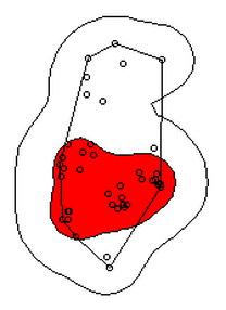
I don’t know about your data, but the href method basically doubles the home range estimate for my snakes. My Snake 1 has a 100% MCP of 10.3, and a 95% UD of 23.4… it’s almost as if Row and Blouin-Demers were onto something… Anyway, let’s visualize everything. Note how the 95% UD (red polygon) looks a lot like the yellow heat signature in the raster image from earlier (that's no coincidence).
plot(getverticeshr(ud,percent=95)) #graph the 95% kernel to the plot
plot(getverticeshr(ud,percent=50),col="red",add=TRUE) #add the 50% kernel to the plot
plot(mcp(s1xy,percent=100),add=T) #add the 100% mcp to the plot
plot(s1xy,cex=.75,pch=1,add=TRUE) #add the gps points
ud <- kernelUD(s1xy,h="href") #calculate and save the utilization distribution
ver <- getverticeshr(ud,percent=95)$area #find and save the 95% utilization distribution
kern <- kernel.area(ud, percent = seq(20, 95, by = 5)) #find and save the ud for 20 - 95%
ver #view the 95% ud area
kern #view the areas for the 20% ud up to the 95% ud by increments of 5
I don’t know about your data, but the href method basically doubles the home range estimate for my snakes. My Snake 1 has a 100% MCP of 10.3, and a 95% UD of 23.4… it’s almost as if Row and Blouin-Demers were onto something… Anyway, let’s visualize everything. Note how the 95% UD (red polygon) looks a lot like the yellow heat signature in the raster image from earlier (that's no coincidence).
plot(getverticeshr(ud,percent=95)) #graph the 95% kernel to the plot
plot(getverticeshr(ud,percent=50),col="red",add=TRUE) #add the 50% kernel to the plot
plot(mcp(s1xy,percent=100),add=T) #add the 100% mcp to the plot
plot(s1xy,cex=.75,pch=1,add=TRUE) #add the gps points
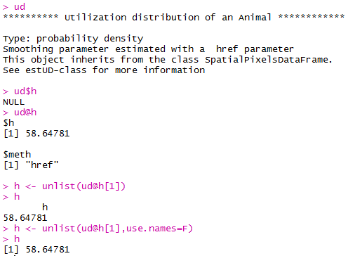
Up until now, we haven’t actually addressed the point of this blog, the h value. How do we get the H value? We pull it from the results of the kernelUD function, which we named ud. If you try to get it by typing in ud, you get nothing ostensibly useful. If you try ud$h, and you literally get nothing. However, ud@h gives you a list containing the value of h, and the method used to calculate it. We want to use the h value later, so we pull it out and store it as a vector. You need to include the use.names=F, or it also includes an h, and we can’t do math with a dumb letter tagging along. The [1] indicates we only want the first item in the list.
2019 update: a lot of these "weird" steps now make a lot of sense as I've advanced as a programer, but I'm going to leave up my colorful laguage because I'm sure new programers can relate to my past frustration!
h <- unlist(ud@h[1],use.names=F) #find the smoothing factor from the utilization distribution
h #view the smoothing parameter
The following part is clunky, and there is probably a better way to do it. In fact, I figured out a better way to do it while I was not day dreaming in class on Tuesday, but then I forgot. So it goes. Basically, we create a matrix, turn it into a data frame, and give the columns names. I’m pretty sure you can just create the data frame without creating a matrix first and give it column names, all in one line of code, so maybe I’ll fix this in the future.
2019 update: I haven't had to use this code recently, but I now think the which() command would be more useful and save a lot of time and effort.
output <- matrix(ncol=2, nrow=h) #create a matrix to fill with home range and smoothing factor values
output <- data.frame(output) #turn it into a dataframe
colnames(output) <- c("h","hr") #add column names
Ok, I’m pretty proud of the following code. It’s a simple loop, but it’s my loop and I love it. It starts by creating a vector called ud_loop, which is the kernelUD function again, but instead of using the href smoothing method, it calculates the ud with the number 1 and stores it in the dataframe we created. Then, it populates the second column of the dataframe with the area of the 95% UD. The loop does this until it calculates the 95% UD with a smoothing factor equal to that used by the href method. Some notes on the code: tryCatch is used to keep the code from stopping if an error or NA pops out; this will happen for certain small values of h. getverticeshr calculates the 95% UD by default, which is why we didn’t specify it. Finally, the +s are used when code wraps to the next line.
2019 update: I'm not longer very proud of this clunky code, but I am proud of the creativity that went into it.
for (i in 1:h) { #start the loop to find smoothing factor values
+ ud_loop <- tryCatch(kernelUD(s1xy,h=i),error=function(err) NA) #trycatch allows loop to progress despite NAs
+ output[i,1]=i #fill first column in dataframe
+ output[i,2]=tryCatch(getverticeshr(ud_loop)$area,error=function(err) NA) #fill second column in dataframe
+ } #end loop
plot(output,type="l",lwd=2) #graph of home range against smoothing factor
abline(s1_homerange,0) #add a line at the 100% mcp homerange value
hvalue <- locator(n=1)$x #physically click on the intersection between the two lines on the graph, which saves the smoothing factor value associated with the 100% mcp
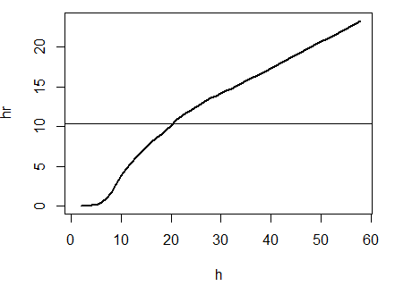
hvalue #print the smoothing factor
[1] 20.3
And there you have it! You can now plug that smoothing value back into the UD command. As you can see, the using the custum smoothing value gives you a 95% kernel that is the same size (or aprox the same size) as the 100% MCP. Note that the output below looks different because I changed the visual settings for Rstudio. This is purely aesthetic.
ud2 <- kernelUD(s1xy,h=hvalue) #calculate the new utilization distribution
ver2<-getverticeshr(ud2,percent=95)$area #find the new 95% utilization distirbution
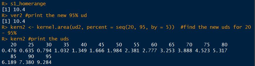
s1_homerange #print the mcp estimate from earlier
ver2 #print the new 95% ud
kern2 <- kernel.area(ud2, percent = seq(20, 95, by = 5)) #view the new uds for 20 - 95%
kern2 #print the uds
ud2 <- kernelUD(s1xy,h=hvalue) #calculate the new utilization distribution
ver2<-getverticeshr(ud2,percent=95)$area #find the new 95% utilization distirbution
s1_homerange #print the mcp estimate from earlier
ver2 #print the new 95% ud
kern2 <- kernel.area(ud2, percent = seq(20, 95, by = 5)) #view the new uds for 20 - 95%
kern2 #print the uds
Finally, let's visualize what we've now done:
plot(getverticeshr(ud2,percent=95)) #view the new 95% kernel
plot(getverticeshr(ud2,percent=50),col="red",add=TRUE) #add the new 50% kernel to the plot
plot(mcp(s1xy,percent=100),add=T) #add the 100% mcp
plot(s1xy,cex=1,pch=21,col="white",add=TRUE)
plot(getverticeshr(ud2,percent=95)) #view the new 95% kernel
plot(getverticeshr(ud2,percent=50),col="red",add=TRUE) #add the new 50% kernel to the plot
plot(mcp(s1xy,percent=100),add=T) #add the 100% mcp
plot(s1xy,cex=1,pch=21,col="white",add=TRUE)
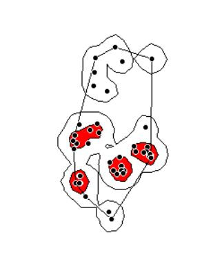
As you can see, the new 50% and 95% UDs are much different than the original 50% HD based on the default href values. These may be similar to or more conservative than your original UD values, but by using this method the results are somewhat more reproducible and likely to be more biologically relevant. Of course, this will also depending on sample size and other factors.
Anyway, hope you enjoyed! Let me know if I can clarify anything or you have any other questions.
Cheers!
Anyway, hope you enjoyed! Let me know if I can clarify anything or you have any other questions.
Cheers!
